Data formats and datasets

Base PDFs

Time PDFs

flarestack.core.time_pdf.box_func(t, t0, t1)

Box function that is equal to 1 between t0 and t1, and 0 otherwise. Equal to 0.5 at to and t1.

Parameters:

• t – Time to be evaluated

• t0 – Start time of box

• t1 – End time of box

Returns:

Value of Box function at t

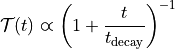
flarestack.core.time_pdf.decay_fct(t, t0, decay_time, truncation=inf)

Decay function that is equal to 0 before t0, equal to 1 at t0 and then decays with a decay time

Parameters:

• t – time to be evaluated

• t0 – start time of the function

• decay_time – decay time

• truncation – truncation time, function will give zero for t < truncation

Returns:

value at t

flarestack.core.time_pdf.decay_fct_integral(tstart, tend, t0, decay_time, truncation=inf)

The integral function of decay_function based on the analytical form

Parameters:

• tstart – float, integrating from

• tend – float, integrating to

• t0 – float, parameter t0 in decay_function, start time of the decay function

• decay_time – float, decay time

• truncation – float, truncation time, decay function will be 0 for t < truncation

Returns:

float

flarestack.core.time_pdf.read_t_pdf_dict(t_pdf_dict)

Ensures backwards compatibility for t_pdf_dict objects

class flarestack.core.time_pdf.TimePDF(t_pdf_dict, livetime_pdf=None)

subclasses: dict[str, object] = {'box': <class 'flarestack.core.time_pdf.Box'>, 'custom_source_box': <class 'flarestack.core.time_pdf.CustomSourceBox'>, 'decay': <class 'flarestack.core.time_pdf.DecayPDF'>, 'detector_on_off_list': <class 'flarestack.core.time_pdf.DetectorOnOffList'>, 'fixed_end_box': <class 'flarestack.core.time_pdf.FixedEndBox'>, 'fixed_ref_box': <class 'flarestack.core.time_pdf.FixedRefBox'>, 'steady': <class 'flarestack.core.time_pdf.Steady'>}

__init__(t_pdf_dict, livetime_pdf=None)

classmethod register_subclass(time_pdf_name)

classmethod create(t_pdf_dict, livetime_pdf=None)

product_integral(t, source)

Calculates the product of the given signal PDF with the season box function. Thus gives 0 everywhere outside the season, and otherwise the value of the normalised integral. The season function is offset by 1e-9, to ensure that f(t1) is equal to 1. (i.e the function is equal to 1 at the end of the box).

Parameters:

• t – Time

• source – Source to be considered

Returns:

Product of signal integral and season

inverse_cumulative(source)

Calculates the inverse cumulative of the time PDF. First, calculates the values for the integral of the signal PDF within the season. Then rescales these values, such that the start of the season yields 0, and then end of the season yields 1. Creates a function to interpolate between these values. Then, for a number between 0 and 1, the interpolated function will return the MJD time at which that fraction of the cumulative distribution was reached.

Parameters:

source – Source to be considered

Returns:

Interpolated function

simulate_times(source, n_s)

Randomly draws times for n_s events for a given source, all lying within the current season. The values are based on an interpolation of the integrated time PDF.

Parameters:

• source – Source being considered

• n_s – Number of event times to be simulated

Returns:

Array of times in MJD for a given source

f(t, source)

sig_t0(source)

Calculates the starting time for the time pdf.

Parameters:

source – Source to be considered

Returns:

Time of PDF start

sig_t1(source)

Calculates the ending time for the time pdf.

Parameters:

source – Source to be considered

Returns:

Time of PDF end

integral_to_infinity(source)

effective_injection_time(source=None)

get_livetime()

get_mjd_conversion()

class flarestack.core.time_pdf.Steady(t_pdf_dict, livetime_pdf=None)

The time-independent case for a Time PDF. Requires no additional arguments in the dictionary for __init__. Used for a steady source that is continuously emitting.

__init__(t_pdf_dict, livetime_pdf=None)

f(t, source)

In the case of a steady source, the signal PDF is a uniform PDF in time. It is thus simply equal to the season_f, normalised with the length of the season to give an integral of 1. It is thus equal to the background PDF.

Parameters:

• t – Time

• source – Source to be considered

Returns:

Value of normalised box function at t

signal_integral(t, source)

In the case of a steady source, the signal PDF is a uniform PDF in time. Thus, the integral is simply a linear function increasing between t0 (box start) and t1 (box end). After t1, the integral is equal to 1, while it is equal to 0 for t < t0.

Parameters:

• t – Time

• source – Source to be considered

Returns:

Value of normalised box function at t

flare_time_mask(source)

In this case, the interesting period for Flare Searches is the entire season. Thus returns the start and end times for the season.

Returns:

Start time (MJD) and End Time (MJD) for flare search period

effective_injection_time(source=None)

Calculates the effective injection time for the given PDF. The livetime is measured in days, but here is converted to seconds.

Parameters:

source – Source to be considered

Returns:

Effective Livetime in seconds

raw_injection_time(source)

Calculates the ‘raw injection time’ which is the injection time assuming a detector with 100% uptime. Useful for calculating source emission times for source-frame energy estimation.

Parameters:

source – Source to be considered

Returns:

Time in seconds for 100% uptime

sig_t0(source)

Calculates the starting time for the window, equal to the source reference time in MJD minus the length of the pre-reference-time window (in days).

Parameters:

source – Source to be considered

Returns:

Time of Window Start

sig_t1(source)

Calculates the starting time for the window, equal to the source reference time in MJD plus the length of the post-reference-time window (in days).

Parameters:

source – Source to be considered

Returns:

Time of Window End

class flarestack.core.time_pdf.Box(t_pdf_dict, season)

The simplest time-dependent case for a Time PDF. Used for a source that is uniformly emitting for a fixed period of time. Requires arguments of Pre-Window and Post_window, and gives a box from Pre-Window days before the reference time to Post-Window days after the reference time.

__init__(t_pdf_dict, season)

sig_t0(source)

Calculates the starting time for the window, equal to the source reference time in MJD minus the length of the pre-reference-time window (in days).

Parameters:

source – Source to be considered

Returns:

Time of Window Start

sig_t1(source)

Calculates the starting time for the window, equal to the source reference time in MJD plus the length of the post-reference-time window (in days).

Parameters:

source – Source to be considered

Returns:

Time of Window End

f(t, source=None)

In this case, the signal PDF is a uniform PDF for a fixed duration of time. It is normalised with the length of the box in LIVETIME rather than days, to give an integral of 1.

Parameters:

• t – Time

• source – Source to be considered

Returns:

Value of normalised box function at t

signal_integral(t, source)

In this case, the signal PDF is a uniform PDF for a fixed duration of time. Thus, the integral is simply a linear function increasing between t0 (box start) and t1 (box end). After t1, the integral is equal to 1, while it is equal to 0 for t < t0.

Parameters:

• t – Time

• source – Source to be considered

Returns:

Value of normalised box function at t

flare_time_mask(source)

In this case, the interesting period for Flare Searches is the period of overlap of the flare and the box. Thus, for a given season, return the source and data

Returns:

Start time (MJD) and End Time (MJD) for flare search period

effective_injection_time(source=None)

Calculates the effective injection time for the given PDF. The livetime is measured in days, but here is converted to seconds.

Parameters:

source – Source to be considered

Returns:

Effective Livetime in seconds

raw_injection_time(source)

Calculates the ‘raw injection time’ which is the injection time assuming a detector with 100% uptime. Useful for calculating source emission times for source-frame energy estimation.

Parameters:

source – Source to be considered

Returns:

Time in seconds for 100% uptime

class flarestack.core.time_pdf.FixedRefBox(t_pdf_dict, season)

The simplest time-dependent case for a Time PDF. Used for a source that is uniformly emitting for a fixed period of time. In this case, the start and end time for the box is unique for each source. The sources must have a field “Start Time (MJD)” and another “End Time (MJD)”, specifying the period of the Time PDF.

__init__(t_pdf_dict, season)

sig_t0(source=None)

Calculates the starting time for the window, equal to the source reference time in MJD minus the length of the pre-reference-time window (in days).

Parameters:

source – Source to be considered

Returns:

Time of Window Start

sig_t1(source=None)

Calculates the starting time for the window, equal to the source reference time in MJD plus the length of the post-reference-time window (in days).

Parameters:

source – Source to be considered

Returns:

Time of Window End

class flarestack.core.time_pdf.FixedEndBox(t_pdf_dict, season)

The simplest time-dependent case for a Time PDF. Used for a source that is uniformly emitting for a fixed period of time. In this case, the start and end time for the box is the same for all sources.

__init__(t_pdf_dict, season)

sig_t0(source=None)

Calculates the starting time for the window, equal to the source reference time in MJD minus the length of the pre-reference-time window (in days).

Parameters:

source – Source to be considered

Returns:

Time of Window Start

sig_t1(source=None)

Calculates the starting time for the window, equal to the source reference time in MJD plus the length of the post-reference-time window (in days).

Parameters:

source – Source to be considered

Returns:

Time of Window End

get_livetime()

get_mjd_conversion()

class flarestack.core.time_pdf.CustomSourceBox(t_pdf_dict, season)

The simplest time-dependent case for a Time PDF. Used for a source that is uniformly emitting for a fixed period of time. In this case, the start and end time for the box is unique for each source. The sources must have a field “Start Time (MJD)” and another “End Time (MJD)”, specifying the period of the Time PDF.

__init__(t_pdf_dict, season)

sig_t0(source)

Calculates the starting time for the window, equal to the source reference time in MJD minus the length of the pre-reference-time window (in days).

Parameters:

source – Source to be considered

Returns:

Time of Window Start

sig_t1(source)

Calculates the starting time for the window, equal to the source reference time in MJD plus the length of the post-reference-time window (in days).

Parameters:

source – Source to be considered

Returns:

Time of Window End

class flarestack.core.time_pdf.DetectorOnOffList(t_pdf_dict, livetime_pdf=None)

TimePDF with predefined on/off periods. Can be used for a livetime function, in which observations are divided into runs with gaps. Can also be used for e.g pre-defined interesting period for a variable source.

__init__(t_pdf_dict, livetime_pdf=None)

f(t, source=None)

livetime_f(t, source=None)

sig_t0(source=None)

Calculates the starting time for the time pdf.

Parameters:

source – Source to be considered

Returns:

Time of PDF start

sig_t1(source=None)

Calculates the ending time for the time pdf.

Parameters:

source – Source to be considered

Returns:

Time of PDF end

parse_list()

get_livetime()

get_mjd_conversion()

signal_integral(t, source=None)

inverse_cumulative(source=None)

Calculates the inverse cumulative of the time PDF. First, calculates the values for the integral of the signal PDF within the season. Then rescales these values, such that the start of the season yields 0, and then end of the season yields 1. Creates a function to interpolate between these values. Then, for a number between 0 and 1, the interpolated function will return the MJD time at which that fraction of the cumulative distribution was reached.

Parameters:

source – Source to be considered

Returns:

Interpolated function

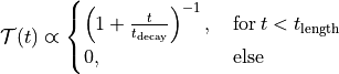
class flarestack.core.time_pdf.DecayPDF(t_pdf_dict, season)

Describing a decaying emission as expected for interacting supernovae (type IIn) following

Zirakashvili, V.N., und V.S. Ptuskin. „Type IIn supernovae as sources of high energy astrophysical neutrinos“. Astropart. Phys. 78 (2016): 28–34. https://doi.org/10.1016/j.astropartphys.2016.02.004.

The elements in the t_pdf_dict are

• decay_time: in the equation above

• decay_length: A time after which is truncated such that

__init__(t_pdf_dict, season)

decay_function(t, t0)

decay_integral(a, b, t0)

sig_t0(source)

Gives the start time of the signal from a source. If the start time lies within the season, the start time is the source’s “ref_time_mjd”. If not it”s the start of the season. :param source: source to be considered :return: time of signal start

sig_t1(source)

Gives the end time of a signal. For an endless decay, that’s just the end of the season. If the decay length is not infinite, the signal might end before the season ends. :param source: source to be considered :return: end time of signal

signal_integral(t, source)

Gives the integrated signal using decay_fct_integral() :param t: float or array like :param source: the sources to be considered :return: float

effective_injection_time(source=None)

Calculates the effective injection time for the given PDF. The livetime is measured in days, but here is converted to seconds.

Parameters:

source – Source to be considered

Returns:

Effective Livetime in seconds

raw_injection_time(source)

Calculates the ‘raw injection time’ which is the injection time assuming a detector with 100% uptime. Useful for calculating source emission times for source-frame energy estimation.

Parameters:

source – Source to be considered

Returns:

Time in seconds for 100% uptime

f(t, source=None)

In this case the PDF is the decay function, normalized to the integral over livetime :param t: float or array_like, Time :param source: Source to be considered :return: Value of normalised box function at t

Energy PDFs

This script contains the EnergyPDF classes, that are used for weighting events based on a given energy PDF.

flarestack.core.energy_pdf.read_e_pdf_dict(e_pdf_dict)

Ensures backwards compatibility of e_pdf_dict objects.

Parameters:

e_pdf_dict – Energy PDF dictionary

Returns:

Updated Energy PDF dictionary compatible with new format

class flarestack.core.energy_pdf.EnergyPDF(e_pdf_dict)

A base class for Energy PDFs.

subclasses: dict[str, object] = {'power_law': <class 'flarestack.core.energy_pdf.PowerLaw'>, 'spline': <class 'flarestack.core.energy_pdf.Spline'>}

__init__(e_pdf_dict)

constructor :param e_pdf_dict:

classmethod register_subclass(energy_pdf_name)

Adds a new subclass of EnergyPDF, with class name equal to “energy_pdf_name”.

classmethod create(e_pdf_dict)

static f(energy)

integrate_over_E(f, lower=None, upper=None)

Uses Newton’s method to integrate function f over the energy range. By default, uses 100 GeV to 10 PeV, unless otherwise specified. Uses 1000 logarithmically-spaced bins to calculate integral.

Parameters:

• f – Function to be integrated

• lower – Lower bound for integration

• upper – Upper bound for integration

Returns:

Integral of function

static integrate(f, lower, upper)

piecewise_integrate_over_energy(f, lower=None, upper=None)

Uses Newton’s method to integrate function f over the energy range. By default, uses 100 GeV to 10 PeV, unless otherwise specified. Uses 1000 logarithmically-spaced bins to calculate integral.

Parameters:

• f – Function to be integrated

• lower – Lower bound for integration

• upper – Upper bound for integration

Returns:

Integral of function bins

static piecewise_integrate(f, lower, upper)

flux_integral(lower=None, upper=None)

Integrates over energy PDF to give integrated flux (dN/dT)

fluence_integral(lower=None, upper=None)

Performs an integral for fluence over a given energy range. This is gives the total energy per unit area per second that is radiated.

return_energy_parameters()

simulate_true_energies(n_s)

class flarestack.core.energy_pdf.PowerLaw(e_pdf_dict=None)

A Power Law energy PDF. Takes an argument of gamma in the dictionary for the init function, where gamma is the spectral index of the Power Law.

__init__(e_pdf_dict=None)

Creates a PowerLaw object, which is an energy PDF based on a power law. The power law is generated from e_pdf_dict, which can specify a spectral index (Gamma), as well as an optional minimum energy (E Min) and a maximum energy (E Max)

Parameters:

e_pdf_dict – Dictionary containing parameters

weight_mc(mc, gamma=None)

Returns an array containing the weights for each MC event, given that the spectral index gamma has been chosen. Weights each event as (E/GeV)^-gamma, and multiplies this by the pre-existing MC oneweight value, to give the overall oneweight.

Parameters:

• mc – Monte Carlo

• gamma – Spectral Index (default is value in e_pdf_dict)

Returns:

Weights Array

f(energy)

flux_integral(e_min=None, e_max=None)

Integrates over energy PDF to give integrated flux (dN/dT)

fluence_integral(e_min=None, e_max=None)

Performs an integral for fluence over a given energy range. This is gives the total energy per unit area per second that is radiated.

return_energy_parameters()

return_injected_parameters()

class flarestack.core.energy_pdf.Spline(e_pdf_dict={})

A Power Law energy PDF. Takes an argument of gamma in the dictionary for the init function, where gamma is the spectral index of the Power Law.

__init__(e_pdf_dict={})

Creates a PowerLaw object, which is an energy PDF based on a power law. The power law is generated from e_pdf_dict, which can specify a spectral index (Gamma), as well as an optional minimum energy (E Min) and a maximum energy (E Max)

Parameters:

e_pdf_dict – Dictionary containing parameters

weight_mc(mc)

Returns an array containing the weights for each MC event, given that the spectral index gamma has been chosen. Weights each event using the energy spline, and multiplies this by the pre-existing MC oneweight value, to give the overall oneweight.

Parameters:

mc – Monte Carlo

Returns:

Weights Array

Spatial PDFs

Composite PDF Objects

Injector

Log Likelihood

Utils

IceCube Utils

Submitter